What is Amortized Analysis?

In amortized analysis, we average the time needed to perform a sequence of data structure operations. By this method, we can show that the average cost of an operation is small, even if we have a single operation within the sequence which might be expensive. Amortized analysis guarantees the average performance of each operation in the worst case.

There are three common techniques used in amortized analysis, which are,

1. Aggregate analysis
2. Accounting method
3. Potential method

Aggregate Analysis

In this method we consider a sequence of n operations and take the worst case time as T(n) in total. Now the average cost, or amortized cost, per operation will be T(n)/n.

Note: This amortized cost applies for each operation, even when there are several types of operations within the sequence of operations.

Example

Let’s consider a stack with operations Push, Pop and Multipop.

• Push(S, x) – Push object x to stack S. Takes O(1) time.
• Pop(S) – Pop (remove) the element on top of the stack and return it. Takes O(1) time.
• Multipop(S, k) – Remove the k top objects of the stack S, popping the entire stack if the stack contains fewer than k elements. If the stack contains s elements, then the running time will be min(k, s).

Multipop(S, k)

while not Stack-Empty(S) and k>0

Pop(S)

k = k – 1

Now consider a sequence of n Push, Pop and Multipop operations on an initially empty stack.

Worst case cost of Multipop operation in the sequence will be O(n) as there at most n elements in the stack. The worst case time for any stack operation will be O(n). Hence a sequence of n operations with order O(n) will take O(n²) time. This is not a tight bound.

Using aggregate analysis we can obtain a better upper bound considering the sequence of operations. We can say that the sequence of n Push, Pop and Multipop operations can cost at most O(n). This is because we can call Pop function (including the Pop calls in Multipop) for each element at most once, as we push them on to the stack.

The average cost of an operation is O(n)/n = O(1)

In aggregate analysis, the amortized cost of each operation is the average cost. Hence, the three stack operations have an amortized cost of O(1).

Accounting Method

In this method we assign different charges for operations. Some operations charge more or less than their actual cost. The amount we charge an operation is called the amortized cost. When the amortized cost of an operation exceeds its actual cost, the difference is assigned to the specific objects in the data structure as credit. Credits can pay for operations which have amortized cost less than the actual cost.

Example

Let the cost of the i^th operation be c_i and its amortized cost be ĉ_i. Then for all the n operations in the sequence, the following should hold.

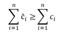
The sum of amortized costs should be greater than or equal to the sum of actual costs. Total amortized cost is an upper bound for the total actual cost.

Let’s consider the same stack example as before. The actual costs of the operations are as follows. The stack contains s elements.

• Push = 1
• Pop = 1
• Multipop(S, k) = min(k, s)

Let’s assign the amortized costs for each of these operations as follows.

• Push = 2
• Pop = 0
• Multipop(S, k) = 0

When we push an element to the stack, we use 1 unit to pay for the actual cost and are left with credit of 1 unit. This credit is left with the pushed element. This credit serves as payment for the cost of popping it from the stack. When we pop an element, we charge the operation nothing and pay the actual cost from the credit stored in that element. The same can be applied for the Multipop function.

When we perform n operations, the total amortized cost will be O(n).

Potential Method

Instead of storing the extra cost as credit, the potential method represents the extra cost as potential energy or just potential.

We perform n operations, starting with an initial data structure D₀. Let c_i be the cost of the i^th operation and D_i be the data structure that results after performing the i^th operation to the data structure D_i-1.

A potential function ɸ maps D_i to a real number ɸ(D_i), known as the potential of D_i. ɸ is defined such that it hold the following two properties.

• ɸ(D₀) = 0
• ɸ(D_i) >= 0

The amortized cost ĉ_i of the i^th operation with respect to the potential function ɸ is defined as,

ĉ_i = Actual cost + Change in potential

ĉ_i = c_i + ɸ(D_i) – ɸ(D_i-1)

Total amortized cost over the n operations will be,

Example

Let’s get back to the stack example. We can define potential function ɸ as the number of objects in the stack. For the initially empty stack D₀ we have ɸ(D₀) = 0. The number of objects in the stack cannot be a negative value. Hence, ɸ(D_i) >= 0.

Now let’s compute the amortized cost for each operation. Consider the i^th operation is performed on a stack with s elements.

For a Push operation with actual cost as 1,

ĉ_i = c_i + ɸ(D_i) – ɸ(D_i-1)

ĉ_i = 1 + (s+1) – s = 2

For a Pop operation with actual cost as 1,

ĉ_i = c_i + ɸ(D_i) – ɸ(D_i-1)

ĉ_i = 1 + (s-1) – s = 0

For a Multipop(S, k) operation with actual cost as k’ = min(k, s)

ĉ_i = c_i + ɸ(D_i) – ɸ(D_i-1)

ĉ_i = k’ + (s-k’) – s = 0

The amortized cost for each of the three operations is O(1) and the total amortized cost for a sequence of n operations is O(n).

 

References

1. Introduction to Algorithms (Third Edition) by Thomas H. Cormen, Charles E. Leiserson, Ronald L. Livest and Clifford Stein